Introduction
Welcome to the third article of our finance theory series, focused on investment. In our previous article, we explored how we can evaluate assets and portfolios by comparing risk and return metrics. We also discussed the effects of asset allocation on reducing risk and how rational investors select efficient portfolios with the best return-to-risk ratios. Now, let's take a deeper look into the risk metric and the concept of diversification.
Diversification
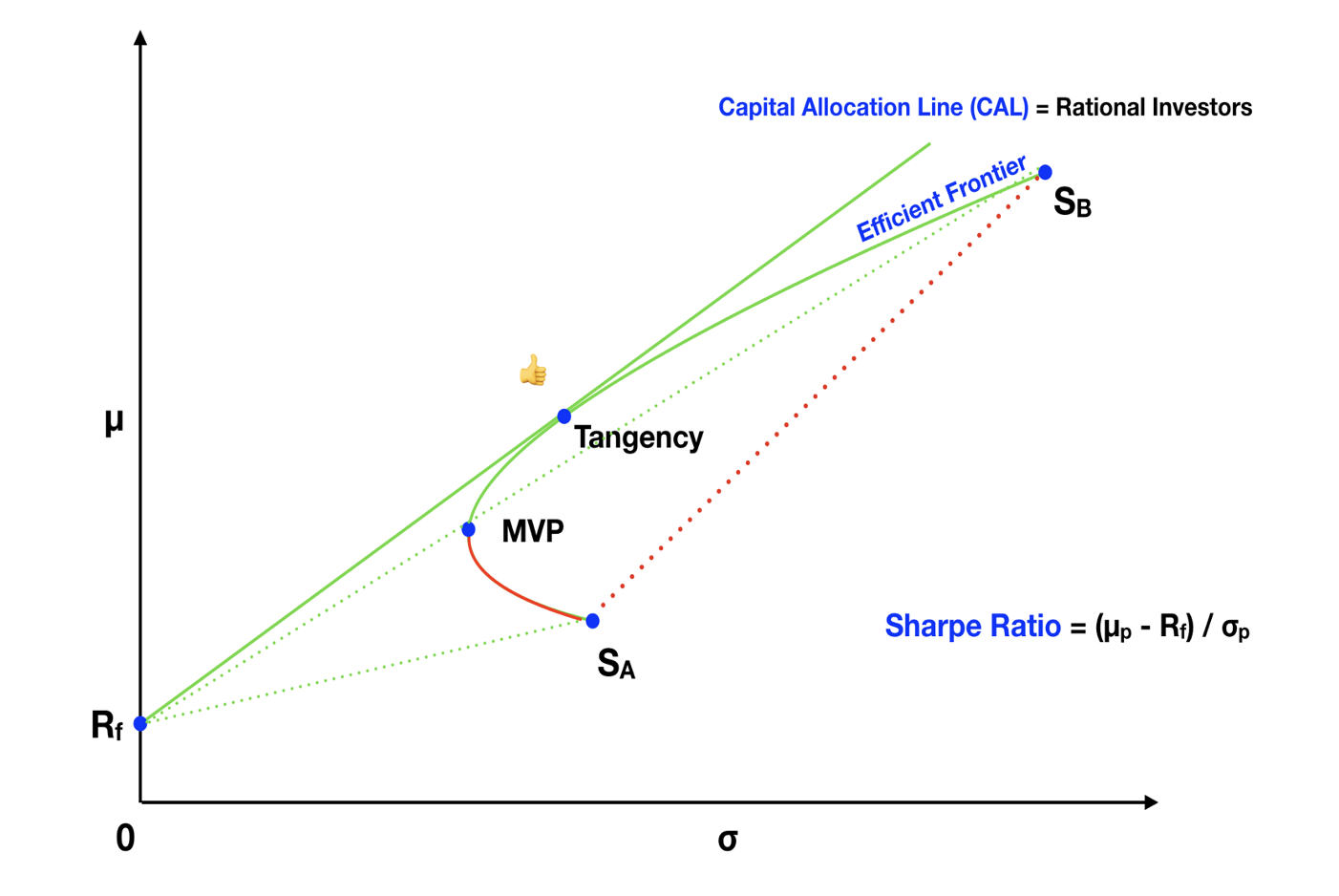
As we've seen, mixing different assets in a portfolio can significantly reduce overall risk. This leads to an important question: Can we aim for a specific portfolio return, while lowering volatility, by adding assets with low correlations? The answer is yes! In our previous discussion involving two risky assets, combining Stock A and Stock B allowed us to create a range of portfolios along the hyperbola curve. Among these portfolios, we identified the Minimum Variance Portfolio (MVP), which boasted much lower volatility than individual assets, such as Stock A or Stock B.

Additionally, we introduced the concept of the Tangency portfolio, which, when combined with a risk-free asset, results in portfolios along the Capital Allocation Line (CAL). This approach lets us maintain the Sharpe ratio, a measure of portfolio efficiency, while fine-tuning risk to suit our preferences. Consequently, we can choose a portfolio along the CAL that offers a similar return to Stock A but with significantly lower volatility.
In essence, Stock A contains a portion of risk that can be eliminated. Since this strategy is readily available, there shouldn't be an additional reward for bearing this diversifiable risk. On the flip side, some risk remains immune to diversification. We can't bring risk down to zero! There's no portfolio with the same return as Stock A and zero risk.
Volatility, often synonymous with risk, has two fundamental components. The first is systematic risk, tied to overall economic factors and immune to diversification. The second is idiosyncratic risk, associated with specific firms or industries and reducible through diversification. The key idea is that systematic risk should command a premium, while there should be no premium for idiosyncratic risk.
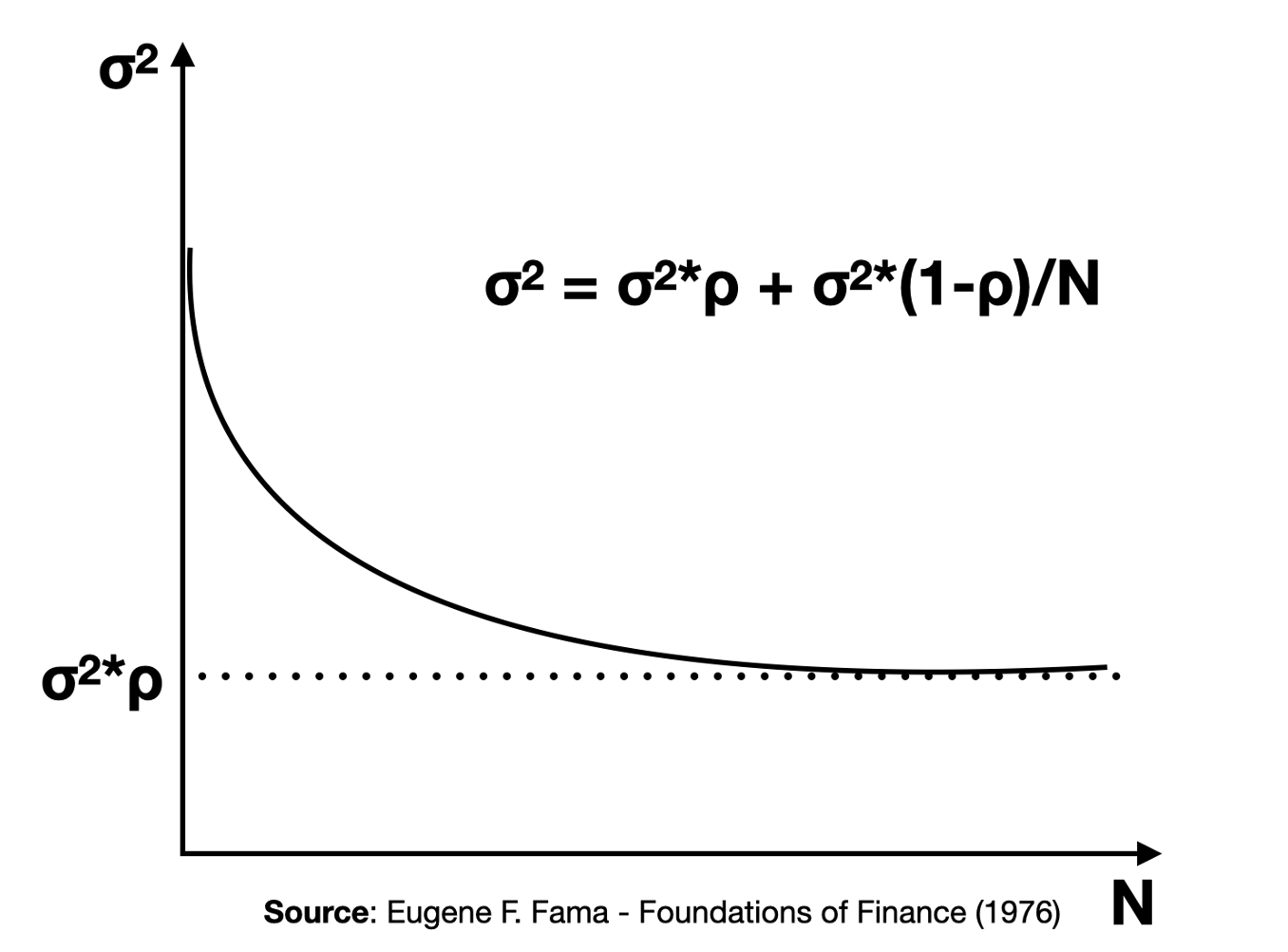
Economist Eugene Fama illustrated the benefits of diversification in his 1976 book, "Foundations of Finance." He computed the expected return and standard deviation of a portfolio with N assets, assuming identical expected returns and standard deviations across all assets. Evidently, the expected return remained constant, since all the individual assets have the same return. The intriguing part comes from analyzing portfolio variance, depicted in the graph below with the x-axis representing the number of assets and the y-axis denoting portfolio variance.

This graph shows that as we add assets to the portfolio, variance decreases rapidly but eventually levels off. It shows that part of portfolio volatility (risk) can be eliminated, while another part can't. Looking at the graph’s equation, we can easily spot both parts of the risk. And again, there should be a premium for bearing undiversifiable risk (systematic risk), whereas diversifiable risk (idiosyncratic risk) should not command a premium.
Empirical data supports the idea that portfolios with more than 20 randomly selected assets tend to be nearly completely diversified, with idiosyncratic risk approaching zero. This example deepens our understanding of asset and portfolio risk and highlights the benefits of diversification.
We've come a long way on our journey to understand asset and portfolio risk. Rational investors, aiming for the highest return per unit of risk, choose portfolios along the Capital Allocation Line (CAL). These portfolios are a blend of the risky Tangency portfolio with the risk-free asset, which is used to calibrate overall risk level. These concepts are the foundation of Modern Portfolio Theory (MPT), introduced by economist Harry Markowitz in a 1952 essay, for which he received the Nobel Prize in Economics in 1990. MPT is one of the most influential portfolio theories and still widely used by institutional investors worldwide.
Markowitz's work paved the way for subsequent research in finance. Assuming rationality and market equilibrium, the Tangency portfolio has a very important mathematical property. The return premium of any portfolio (mean portfolio return minus the risk-free return) divided by its covariance with the Tangency portfolio, is equal to the return premium of the Tangency portfolio divided by its variance. The covariance metric is easily calculated by multiplying the standard deviation of the portfolio, the standard deviation of the Tangency portfolio, and the correlation between the two. Here is the formula:
(μp - Rf) / cov(Rp, RT) = (μT - Rf) / σT2
With a little bit of algebra, we can write the equation in this new form:
(μp - Rf) = (cov(Rp, RT) / σT2) * (μT - Rf)
Where
cov(Rp, RT) = σT * σp * ρpT
and
cov(Rp, RT) / σT2 = β
The rewrite shows that the premium of any asset or portfolio is determined by a specific number, which we call beta (β), times the premium on the Tangency portfolio. You've probably heard about the beta metric before. It relates to the systematic risk, the overall economy risk, the part of the volatility that we cannot diversify.
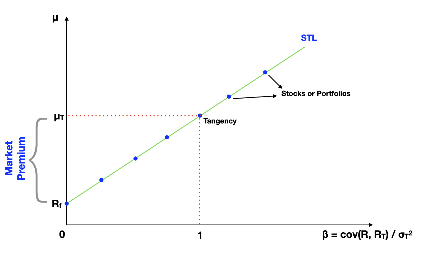
We can also plot this equation on a graph, so we can analyze how returns varies in regards to systematic risk only, instead of using volatility, which is a measure of total risk. On the following graph, we have beta on the x-axis, and return on the y-axis. Our equation is represented by a straight line crossing the y-axis at the risk-free rate.

Looking at both the formula and the graph, we can conclude that the expected return of all assets and portfolios should depend on their respective systematic risk (beta). In addition, the more systematic risk, the higher the yielded return. The returns go up progressively on a straight line, called the Security Tangent Line (STL). The slope of this line is called the Treynor ratio and is expected to remain constant.
Slope of STL = Treynor Ratio = (μp - Rf) / βp = constant
Another important insight from this analyzes relates to the value of assets and portfolios in the market. If we find assets in the market that are delivering higher returns than expected, meaning they're positioned above the STL, they're probably undervalue. There's an additional return that one would gain by investing in it. Whereas assets that deliver a lower return than expected, positioned below the security tangent line, are probably overvalued and not delivering enough return for their risk. These are key insights of another important finance theory, the Capital Asset Pricing Model (CAPM).
The CAPM was created by many scholars who worked on this problem around the same time (Jack Treynor 1961-1962, William F. Sharpe 1964, John Lintner 1965 and Jan Mossin 1966). Some of these scholars also won the Nobel Prize of Economics in 1990. The CAPM had a major influence in how we value assets in the market, from private companies to public stocks. And it's still widely used today.
What's Next
In the fourth article of this series, we'll take a dive deeper into the Tangency portfolio and explore the best approximations available for it in market. If you have comments or feedback about this article, please send us a note at feedback@bearnbull.com. Make sure to also visit BearNBull's website, where you can find more resources to make you a better investor.