Introduction
What’s your portfolio return? Is it enough for the level of risk you are taking? How diversified is your portfolio? Most investors have a hard time answering these questions! Let’s be honest, measuring portfolio performance is complicated. It takes a lot of number crunching and sensible analysis to understand how a portfolio is actually performing and make predictions about future performance.
Whether you are a self-directed investor or you like to delegate your investment decisions to a professional, correctly measuring portfolio performance is a key part of investing, which everyone should be familiar with. Yet, the majority of investment reports and financial applications don’t provide adequate performance metrics. Many investors will end up aggregating data on a custom spreadsheet. The process is cumbersome and prone to errors. For most people, these custom tools never live up to their vision and end up not being used. Lost in this rabbit hole, investors then rely on poor metrics and intuition for decision making.
This series of three articles will explain how you can truly get a hold on your portfolio performance. On part one, we'll discuss key performance metrics. On part two, we’ll introduce more overlooked, yet very important, metrics. We'll also describe in detail how each metric is calculated. Finally on part three, we’ll explore clever ways to present the data, which will help us make better investment decision.
A Taste Of Reality
Here is a real-life scenario: you setup an equity portfolio, with stocks from ten different companies, diversified by sector. One year has passed, you've added two more stocks, and traded a few positions. Now you want to assess your performance and make changes if necessary. Sounds simple, right?
You log into your brokerage or bank website. The market value and initial cost of each asset is available. Great, you know how much you gained or lost! Then, a few questions pop up on your head: Is that good or bad? Could I have done better? You dig for the information and nothing.
You are pretty familiar with spreadsheets, right? You decide to grab the bull by the horn. You download all the transactions to a file in your computer and start crunching the numbers to figure out the portfolio's return. One hour has passed and you realize how painful a task that is.
Calculating return is easy for one asset and no trades, but multiple assets and trading just a few positions make it hard. There are also many ways to calculate actual and expect returns. Which method should you use?
Getting a roadmap

Before diving into the spreadsheet, it's important to reflect on what you are trying to accomplish. Asking the right questions is a great way to start and points us in the right direction. Here are three simple, yet important, questions you might come up with:
- How did the portfolio actually performed?
- Was trading during this period helpful?
- What performance should I expect for this portfolio?
Now that we know where we want to go, we need a roadmap to get there. Let's go over each of these three questions in detail and define the metrics that will help us answer them:
How did the portfolio actually performed?
There are many parts to measuring portfolio performance. For now, let's assume you are already monitoring total value, gains/losses and cashflows of your portfolio, as this information is easily accessible. The next natural step is figuring out your actual portfolio return. There are two main methods for calculating actual return: Money Weighted Rate of Return (MWRR) and Time Weighted Rate of Return (TWRR). Each metric has its own merit, so we need to understand what is being measured and when to use them.
MWRR is an Internal Rate of Return (IRR) of a portfolio, it includes all effects of cash flows during the period. This mean that adding money to or taking money from the portfolio will change this metric. Adding money before a high growth period increases MWRR. Taking money out before a high growth period decreases MWRR. MWRR gives a sense of the performance during the period, but analyzed by itself, it can be quite misleading. There is more weight to the performance when the portfolio is larger, which is where the “money weighted” name comes from. You also can't compare it to any benchmark or to other portfolios, as these might have different cash flows. TWRR on the other hand eliminates any cash flow effect. This means you can use it to compare performance with other portfolios, funds or indexes.
Was trading during this period helpful?
MWRR and TWRR comparison can help us answer our second important question. As you might have guessed. When MWRR is greater than TWRR, we can conclude that cash flows had a positive impact on portfolio performance. And vice versa. Simple! Here is an example of a portfolio with stock from just one company (Apple), to illustrate MWRR and TWRR:
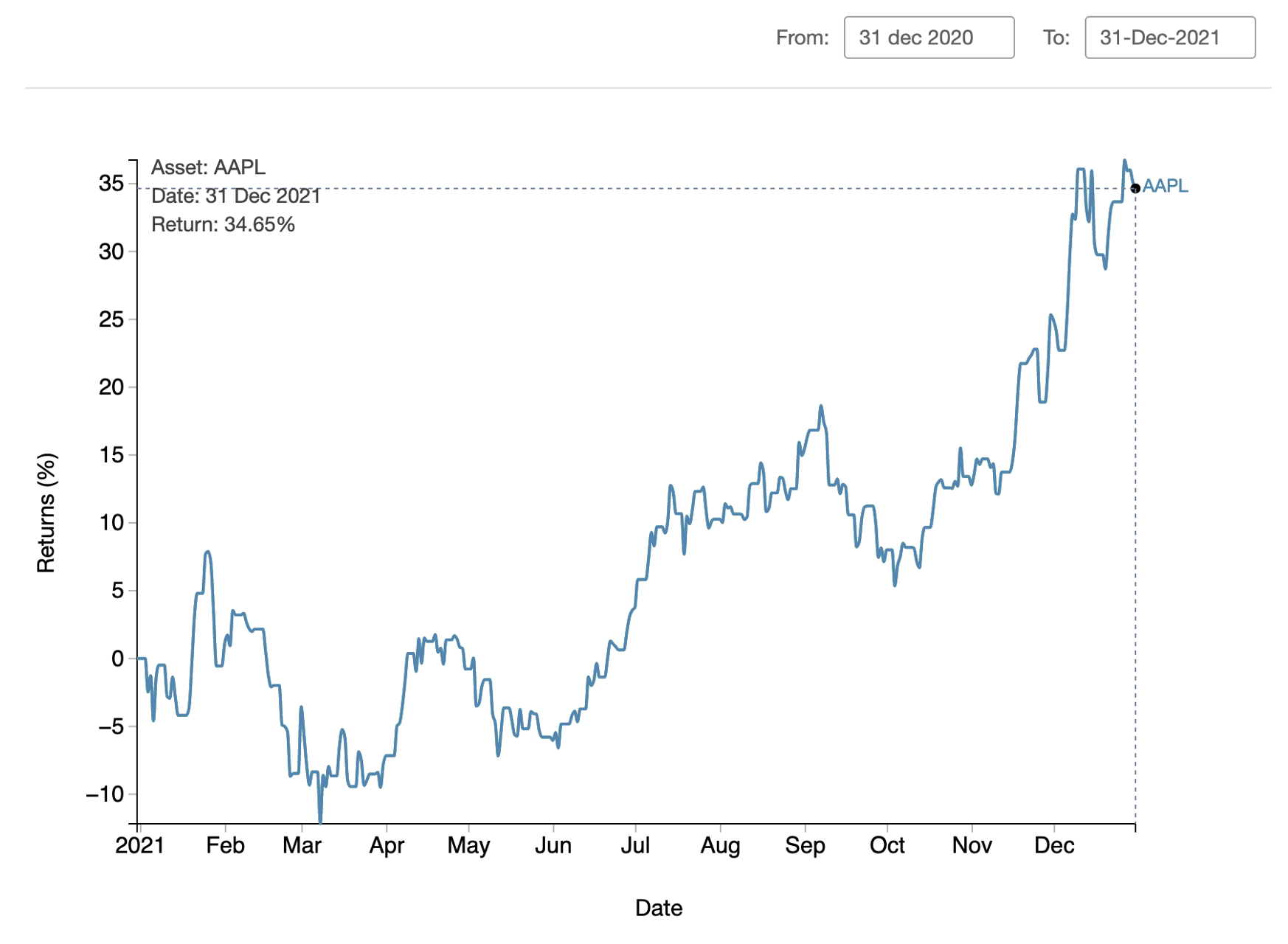
Apple ended 2020 with a stock price of $132.69 ($131.33 Adjusted). At the end of 2021, the stock price was $177.57 ($176.84 Adjusted). In 2021 Apple stock had an impressive return of 34.65%!
Apple 2021 Return = (176.84/131.33) - 1.0 = 34.65%
Let's now imagine three trading scenarios and evaluate the impact on the return metrics:
Scenario 1:
We had one stock of Apple in our portfolio at the beginning of the period and held it throughout the year. In this case, there were no trades during the period, so the TWRR and MWRR returns of our portfolio at the end of the year were both 34.65%, the same return of Apple stock.
Scenario 2:
We had one stock of Apple in our portfolio at the beginning of the period and held it throughout the year. We also bought another Apple stock at the end of the day on Nov 30th, when the price was $165.30. In scenario 2, there is one trade during the period. The TWRR should be unaffected by this trade, since it didn't change the portfolio allocation, so TWRR of our portfolio is still 34.65%. The MWRR on the other hand, is now 40.40%, a significant increase. Since MWRR is greater than TWRR, we can say we timed our trade well, which makes sense, since we bought the stock before a high growth period at the end of the year.
Scenario 3:
We had one stock of Apple in our portfolio at the beginning of the period and held it during the year. We also bought another Apple stock at the end of the day on Dec 10th, when the price was $179.45. A similar scenario with one trade during the period. The TWRR is again unaffected by this trade, so TWRR of our portfolio is still 34.65%. But MWRR is now 31.04%, a significant decrease. MWRR is less than TWRR, which means poor timing on the trade. This also makes sense, since we bought the stock at a higher price than the year end price.
| Scenario | TWRR | MWRR | Trade Impact |
|---|---|---|---|
| 1 | 34.65% | 34.65% | Neutral |
| 2 | 34.65% | 40.40% | Positive |
| 3 | 34.65% | 31.04% | Negative |
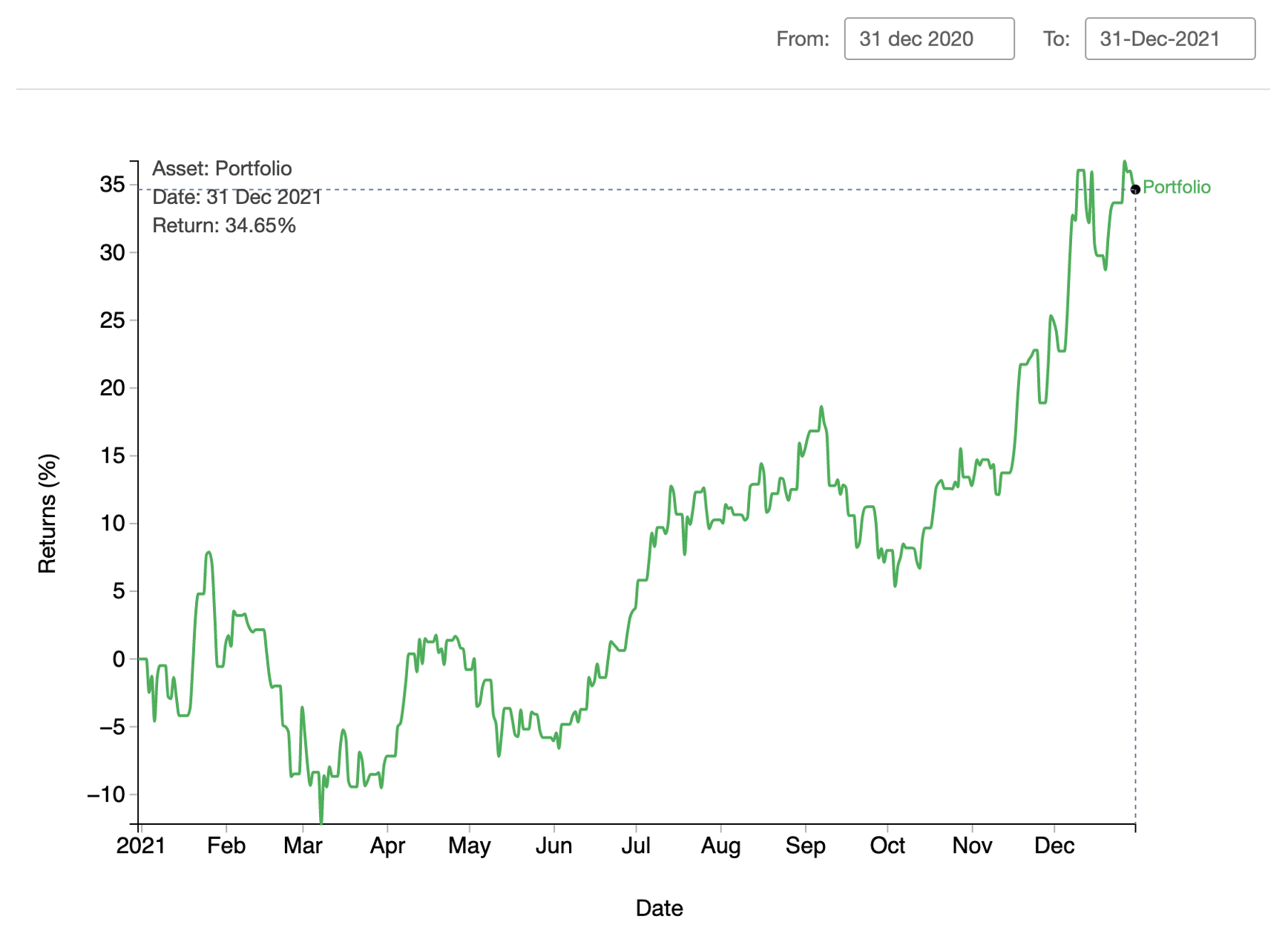
The graphs below show the cumulative return for Apple stock and for a portfolio of Apple stock. The TWRR of our portfolio during 2021 is equivalent to Apple stock's cumulative return on the same period. It also does not change for the different trading scenarios, so we can use it for comparison with other portfolios. Hopefully this example helps us understand the importance of having both TWRR and MWRR in our performance analysis.


What performance should I expect for this portfolio?
Expectation has to do with the future forecast of our performance. We want to come up with a logical estimation of our portfolio return. There are many different ways for estimating returns, but we'll focus on two key methods.
One method is looking at the past. We select a reliable period of data for each asset in our portfolio and calculate returns for a selected frequency, for example, five years of monthly returns. We then average the values out to get an expected return for each asset. A weighted average of all the asset's expected returns, based on the current percentage allocation, is our portfolio expected return.
A second method consists of creating a model to predict the future. There are many models available, but to keeps things simple, we'll focus on the Capital Asset Pricing Model (CAPM). The CAPM says the expected return of an asset is equal to the risk-free rate, plus the beta (market risk metric) times the excess return on the overall market (market return minus risk-free return). Here is the formula:
E(RA) = Rf + βA * (E(Rm) - Rf)
If we have values for the expected market return, risk-free return and beta, we can calculate the asset's expected return. Our portfolio's expected return is again a weighted average of all the asset's expected returns, based on our current percentage allocation. Another approach for this method, is calculating first the beta of the portfolio, which is a weighted average of all the asset betas, based on our current percentage allocation. And then using the CAPM formula to calculate the portfolio expected return. The end result is the same!
A quick side note here, on the CAPM method, we're also looking at past data to estimate market return and beta. In different ways, both methods rely on the past to predict the future. You might be thinking: isn't the past not reliable for guaranteeing future results. And you are right! We cannot blindly believe in these predictions, as the future might unfold very differently than what we expect. Nevertheless, they are good pointers to what has happened and is possible in the future. As to which method we should use, the answer is both. Using both methods gives us a range of possible outcomes to work with.
Conclusion
Knowing how our portfolio actually performed, whether trading was helpful and having a clear vision for what to expect in the future is no easy task. Most investors get lost when assessing their portfolio performance and end up relying only on intuition for decision making. Part one of this portfolio performance series gave us a roadmap to answer some important investment questions. On part two: The Perils Of The Path, we’ll talk about the elephant in the room that we’ve been avoiding and describe in detail how to calculate each metric.