Introduction

Welcome to the fifth article of our finance theory series, focused on investment. In the previous article, we explored the concept of the Tangency portfolio, a key component of rational investing. We discovered that, in a simplified economy example, the Tangency portfolio is equivalent to the market portfolio and is a value-weighted combination of all assets in the market. In this article, we'll delve deeper into asset pricing models, such as the Capital Asset Pricing Model (CAPM) and other multi-risk factor models.

Pricing Assets

Before we talk about asset pricing models, let's recap some essential insights from Modern Portfolio Theory (MPT) and the CAPM. We began with the assumption that financial asset returns follow a normal distribution, allowing us to quantify them by mean and standard deviation. By creating portfolios with different low-correlation assets, we learned that diversification can reduce the total risk of a portfolio (volatility). We saw that part of the total risk is diversifiable (idiosyncratic risk) and is related to specific company/industry. Another part remains undiversifiable (systematic risk) and is linked to the overall economy.

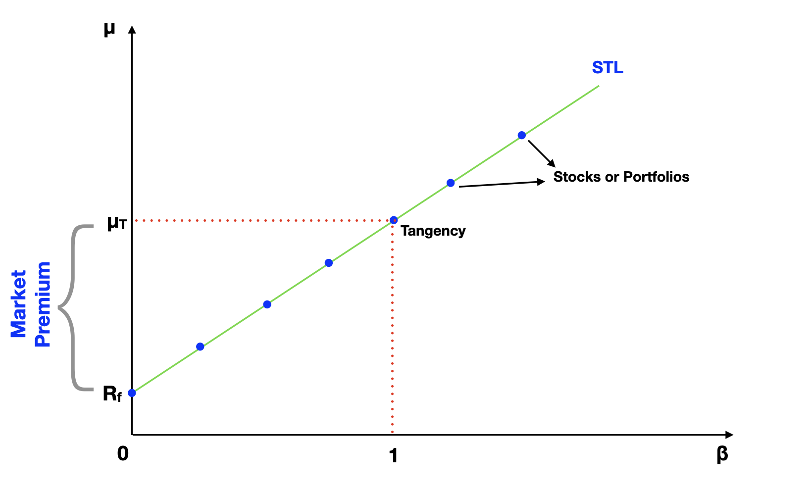
The CAPM provides a framework for pricing assets based on their beta, a measure of systematic risk. The following graph exemplifies the relationship between the expected return of an asset or portfolio and its beta (systematic risk):

The CAPM predicts that all assets should be lined up on the Security Tangent Line (STL). The CAPM equation is the result a linear regression, where the premium return of any portfolio or asset is the dependent variable, and the premium on the Tangency portfolio is the independent variable.

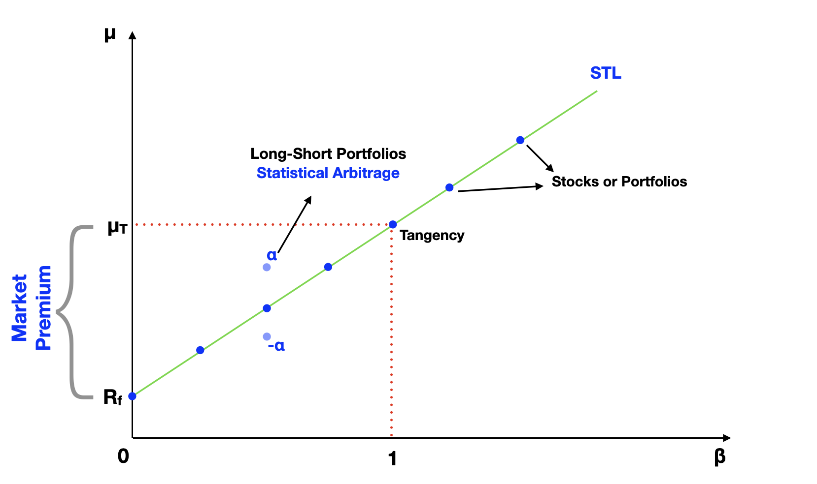
If the CAPM is correct, we expect the alpha constant (α) to be zero. If we find assets in the market that show either positive or negative alpha, we can assume they are mispriced. An asset is undervalued if alpha is positive or overvalued if alpha is negative.

We can arbitrage and extract the alpha over a time period using a long-short portfolio strategy. For example, we can buy the undervalued asset (long) and sell (short) a portfolio at the STL with similar beta. This is called statistical arbitrage, which is different than a perfect arbitrage opportunity since there's still some known probability that the strategy might fail.

I won't go into the details, but we can calculate the probability of success using the random error component (ε) of the regression. This is a common money-making strategy used by many hedge funds. Although the odds are usually much better than playing in a casino, sometimes the strategy can go wrong and if the bet was too big, potentially bankrupt the hedge fund.

The regression also provides other valuable information such as the Pearson's correlation coefficient, known as the R-squared (R²). It measures the closeness of the data to the regression line or how well the regression explains a set of data. We can interpret it as the percentage of the portfolio or asset return, which is explained by the market return.

The remaining percentage relates to other factors and is spilled over into the epsilon (ε) component of the regression, known as the random error. We can rewrite the R-squared equation in terms of asset variance, which helps dissect the asset's risk into systematic (related to beta) and idiosyncratic (ε) components. The systematic risk is the product of beta squared and the variance of the market. The idiosyncratic risk is the variance of the epsilon component of the regression.

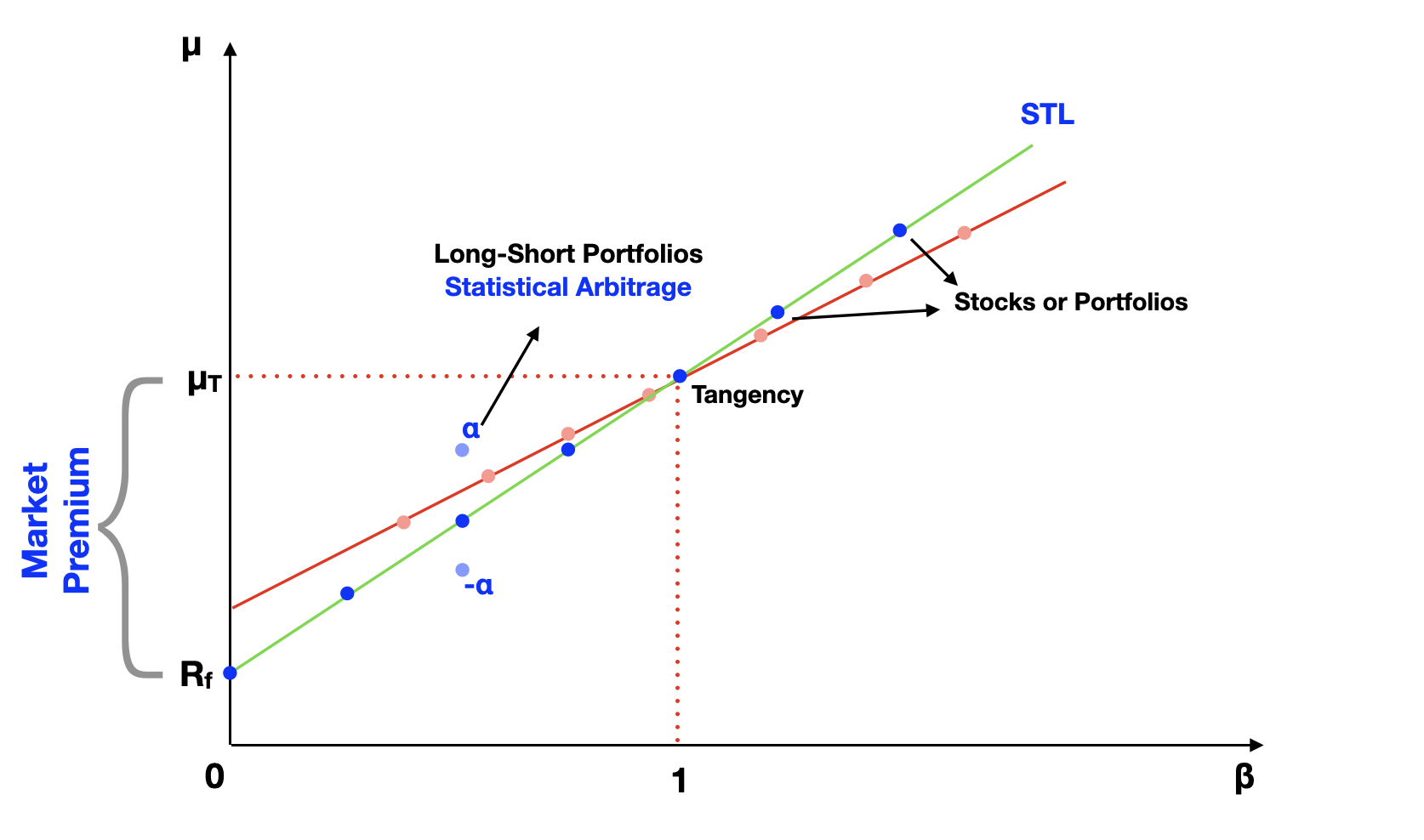
Many finance scholars have tried to test the CAPM using empirical data. Some of the most famous studies are the 1972 studies by Fischer Black, Michael Jensen, and Myron Scholes. And more recently, 1992, the works of Eugene Fama and Kenneth French. They discovered that lower beta assets actually deliver higher returns than expected by the CAPM. And the opposite is true for higher beta assets. From their data, the Security Tangent Line looks flatter, like the red line in the following graph:

These results make many questions the validity of the CAPM. And this is an ongoing debate in finance. How can we prove if the CAPM is correct? There are three hypotheses we can make:

First, we can say the market is unobservable and should include all assets in the whole economy. Since we're using incomplete proxies, such as a total US equity market index, we have an improper measure of market returns. Therefore, we cannot prove that the CAPM is wrong. It could actually be correct if we used the right proxy.

Second, we can assume that the market proxy is good. In this case, the CAPM might be missing other risk factors beyond beta, which can account for the differences in expected returns. Instead of just one beta, which reflects the overall market risk, we should have multiple independent variables in the regression, and therefore, multiple betas.

This second hypothesis led both finance scholars and investors to search for multi-risk factor models. The most famous is probably the Fama-French model, which accounts for three risk factors. In addition to market risk, the model has two additional beta components, one related to the size of the company and another related to the book to market ratio of the company. Fama and French found empirical data showing that small stocks outperform large stocks in the long run, and also that value stocks outperform growth stocks in the long run.

Many people contested Fama and French’s conclusion, saying that it was the result of data mining. Others have taken it further by introducing other factors, such as momentum. We’ve seen a flourishing of four or five factor models. The multi-risk factor models have also contributed to the growth of investing strategies called factor tilting or smart betas, where investors add higher weights to specific risk factors such as company size, which could yield higher returns in the long run, instead of just investing in the market portfolio.

And third, we can say the market is inefficient, therefore assets are mispriced and arbitrage has failed to correct the differences.

Solving the hypothesis puzzle is hard! When we find an apparently misprice assets in the market, such as the positive and negative alpha examples, we cannot tell for sure whether the market is inefficient because we don't know if the model is correct. This is called a joint hypothesis problem.

The issue has split finance scholars into two schools of thought. A rational school of thought, which believes in market efficiency and creates models to understand the relationship between return and risk. And a behavioral school of thought, which says markets are inefficient because people make errors in setting prices and arbitrage trading fails to correct them.

• Hypothesis 1: Improper measure of market returns. → Whole Market is Unobservable
• Hypothesis 2: There must be other risk factors! → Multi-Risk Factor Models
• Hypothesis 3: The assets are mispriced. → The Market is Inefficient

What's Next

In the sixth article of this series, we'll talk more about the market efficiency assumption, which is of key importance for understanding how to model the financial markets. If you have comments or feedback about this article, please send us a note at feedback@bearnbull.com. Make sure to also visit BearNBull's website, where you can find more resources to make you a better investor.